Mobius strip parametrization

Recently I thought about a way to parametrize the Mobius strip embedded in 3D.

The intuition was the following:

If someone were to look "down" along the circle of the strip, they would see a circle rotating by 180 degrees.  A circle of this kind in 2D is very simply parameterized by:

$$
x_c(r,\psi) = r \cos(\psi) \\
y_c(r,\psi) = r \sin(\psi)
$$

Now we need to wrap this around a circle.  This would mean that the plane the half-circle sits in should be normal to the tangent vector of the circle in 3D.

I choose to wrap my Mobius strip around the axis z with overall radius $R$.  So I have the parameterization

$$
x = R \cos (\phi) \\
y = R \sin (\phi) \\
z = 0
$$

It's not hard to see that at every point on this circle, two basis vector for the plane normal to the tangent vector is given by:

$$
\hat e_1 = (\cos \phi, \sin \phi, 0) \\
\hat e_2 = (0, 0, 1)
$$

With offset
$$
(R \cos \phi, R \sin \phi)
$$

Together, using the equations for \((x_c, y_c)\), I get the overall parametrization:

$$
x_c(r,\phi)\hat e _1 (2\phi) + y_c(r,\phi) \hat e_2 (2\phi) + (R \cos \phi, R \sin \phi, 0)
$$

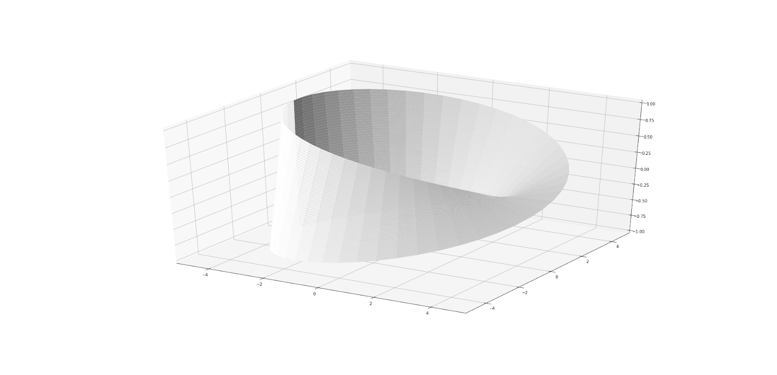
Using matplotlib, I have something like:

import numpy as np
from mpl_toolkits.mplot3d import Axes3D
import matplotlib.pyplot as plt
from matplotlib import interactive
import math
import matplotlib
matplotlib.use('Qt5Agg')

R = 4

def mobius(r, phi):
    x_ = r * math.cos(phi)
    e1 = np.array([math.cos(2*phi), math.sin(2*phi), 0])
    y_ = r * math.sin(phi)
    e2 = np.array([0, 0, 1])
    return x_*e1 + y_*e2 + np.array([R*math.cos(2*phi), R*math.sin(2*phi),0])


# Generate torus mesh
phi = np.linspace(-0.5*np.pi, 0.5*np.pi, 50)
r = np.linspace(-1, 1, 50)
r, phi = np.meshgrid(r, phi)
X = np.ndarray(r.shape)
Y = np.ndarray(r.shape)
Z = np.ndarray(r.shape)
for (x,y) , r_scalar in np.ndenumerate(r):
    phi_scalar = phi[x,y]
    result = mobius(r_scalar, phi_scalar)
    X[x,y] = result[0];
    Y[x,y] = result[1];
    Z[x,y] = result[2];

# Display the mesh
# plt.switch_backend('Qt5Agg')
# %matplotlib qt5
fig = plt.figure()
ax = fig.gca(projection = '3d')
ax.set_xlim3d(-5, 5)
ax.set_ylim3d(-5, 5)
ax.set_zlim3d(-1, 1)
ax.plot_surface(X, Y, Z, color = 'w', rstride = 1, cstride = 1)
plt.show()

Output looks like: